Happy New Year 2016

The year 2015 is ending very shortly.

I wish every readers of my blog an exciting new year ahead that is full of happiness and prosperity.

From my blog statistics, most of my visitors comes from the US and Europe. There is negligible traffic coming from developing countries. This can be correlated to the fact that exploitation of geo-spatial data in developing countries is still in infant stage. On average, I tend to get around 600 visits on my blog, which is not a lot but its good to see that someone actually bothers to read the posts that i wrote. When i get an email from my visitors mentioning that some posts helped them to do things in their professional life, i am over the moon on that day :). 

These are the all-time top 10 posts within my blog that seems to be attracted to many users. Some of the post that I have written in 2010-11 is still very popular among visitors, specially related to ArcGIS. The post related to GIS gets more hits than those related to Remote Sensing. I tend to write less related to GIS posts as I don’t work with GIS day in and day out.  I will write more related to Remote Sensing in coming days. The top ten blogs post are related to MATLAB : 5  ARCGIS: 4 and eCognition: 1. I could not get the posts specific statistics for 2014 from blogger but lately my eCognition related blogs are liked by many visitors. I have made few friends through my blogs which is awesome.

1. KMLcreation using MATLAB
2. Openingmultispectral or hyperspectral ENVI files in MATLAB
3. Convertingraster dataset to XYZ in ARCGIS !!
4. UtilizingNumpy to perform complex GIS operation in ARCGIS 10
5. Data DrivenMap Book in ArcGIS 10
6. ArcPy :Python scripting in ArcGIS 10
7. MATLAB GUIfor 3D point generation from SR 4000 images
8. MATLABtutorial: Dividing image into blocks and applying a function
9. MATLABTutorial: Finding center pivot irrigation fields in a high resolution image
10. eCognitionTutorial: Finding trees and buildings from LiDAR with limited information

eCognition Tutorial: How to find segments which have lower mean value to the neighbouring segments with additional condition to class?

I have segmented data, classified into two classes: 1, 2. I would like to find segments into the 1 class which are adjacent to the 2 class and have lower mean value. The one condition should be: Existence of 2 > 0, but how to combine it with information about lower mean value of segment?

This is a problem posted in the eCognition community by one of the user. One of the core strength of OBIA is to incorporate contextual information and class related information in the process which is difficult with pixel-based approaches. Here the class of interest has to satisfy two contextual class related information:

1)      It must be bordering the class 2

2)      It must be class 1 and must have lower mean value

The Problem

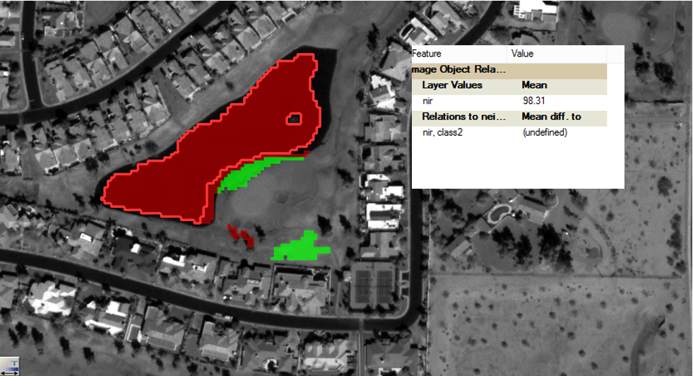
For this problem, we have to make a class related feature ( Class-Related features >  Relation to neigbor objects > Mean diff. to  ) that is based on a layer of interest and class. For demonstration purpose I will be using NIR layer. So the feature that is created is “Mean diff to nir, class 2”. In the following figure, we can see the feature “Mean diff to nir, class 2” on the right side. In the figure, objects that are not bordering the class 2 have undefined value (red), the objects that are bordering the class 2 and have lower “Mean diff to nir, class 2”,  have smaller value (darker) and the objects that are bordering the class 2 and have higher “Mean diff to nir, class 2”,  have higher value (brighter).




The custom feature

 

For better illustration I have attached some figures that also show values for “Mean diff to nir, class 2” feature.

Class 2 object

Class 1 object not bordering class 2

Class 2 objects bordering Class 1

Unclassified object bordering Class 1

  

Afterwards, the extraction of objects of interest is straight forward. We use assign class algorithm for that purpose.

 

Assign class

The solution. Pink color represent objects we are attempting to extract.

 

Nepal, Mr. Modi and Petrol stations

I know that I haven’t posted for a very long time for now. Please accept my sincere apology. There have been lots of things that going around in my life. I have moved to my home country Nepal after almost 10 years of stay in Europe in February 2015.  Unfortunately, a big earthquake hit Nepal on 25^th April 2015 that has severely affected many peoples in Nepal. Around 10,000 peoples were dead.  Many people lost their relatives and belongings. Everybody suffered by wrath of the mighty Earthquake.  

Things started to become normal after several months and suddenly Mr. Modi, the prime minister of India Modi-fied the life of Nepalese people who were attempting to enjoy their day to day normal life and were enthralled by newly formulated constitution.  Nepal was slapped by an unofficial blockade from India limiting supply of essential commodities and fuel in Nepal. Being a landlocked country, Nepal solely relies on India for its need of fuel. Being a sovereign country, Nepal has every right to decide what is right for the people of Nepal and to promulgate constitution that was ratified by over 90 % of constitution assembly members. India did not like some part of the constitution and started the so called “unofficial” blockade since beginning of September 2015.  The interference of India on internal affair of Nepal is totally wrong from any possible angle but surprisingly India thinks that they have every right to bully Nepal. Now, due to the blockade life of a common Nepalese people is very miserable. There is scarcity of cooking gas, no fuel (petrol and diesel) to run vehicles. Miles long queue of vehicles are a normal scene at every nook of the capital, Kathmandu. If someone has 20 liters of petrol or diesel or 2-3 cylinders of cooking gas, then he/she is part of the minority of people in Kathmandu who happily celebrated the ongoing festive season of Dashain and Tihar. For everyone else, days are spent counting numbers of fuel carrying vehicles entering Nepal and queuing at a fuel station on a scorching heat. Things are so bad in Kathmandu and majority of places in Nepal that if you like to irritate someone, just say ‘Did I tell you something, you look like Mr. Modi with that beard’. LOL.

Rambling aside, I was looking for a map of fuel stations in Kathmandu, and no surprise I could not find one. Not even in the official website of Nepal Oil Corporation (NOC) , the sole body that is responsible for import and distribution of fuels within Nepal. I did not even find a simple table list. Shame NOC. So I decided to create one. For the map, I used Open Street Map (OSM) data. The fuel station list may be incomplete as data was gathered from Voluntary GIS (VGIS) approach. For queering the data, Overpass-API was used. Overpass-API is a query language that is used to grab data of interest from OSM. For displaying the map, the power of GIST from GITHUB was used. If you like KML file of the map then click here. I will write a detail post about Overpass-API sometime in future when I will be tired of scolding Mr. Modi for his wrong deeds. For now its everyone’s favorite things to do here in Nepal. Even ladies love it more than watching  Indian drama serials.

MATLAB Tutorial: Finding trees and buildings from LiDAR with limited information using Mathematical Morphology

Coming soon :

Last Pulse

First Pulse

Classification of buildings and tree

Processing TIME: < 1 sec

MATLAB tutorial: Dividing image into blocks and applying a function

Often due to the limitation in memory, we want to divide an image into mxn blocks and process those blocks. If your block processing outputs an image then, you can use blockproc function in MATLAB. But, if processing function outputs points then one can’t use block processing. For that, one has to rely on image indexing to divide image into blocks. So here I will show you how you can divide image into blocks and process those individual blocks for any particular function using indexing. I am going to use block processing for finding pivot irrigation fields detection that was featured in this post. The trick is to apply matrix indexing to get chunk of block data and process them in a sequential manner. 

Here is the original image. We are going to divide it into mxn blocks. With the code you can specify any m or n value.

Original image

Block processing sequential numbering

With the following code, the block processing on individual blocks are performed. Feel free to copy the code and adapt it to your liking. Everything in the code is self-explanatory, so just go through the code line by line and you will understand whats going on.

The output of block processing for original image is as follows:

Block processing of detecting circles 

.

MATLAB Tutorial: Finding center pivot irrigation fields in a high resolution image

In this post, we will be talking about finding circular irrigation fields. The image was download from here. If you want to try, download it and play around. The approach I am using is detection of edges and finding edges that form circular edges. If you have heard of Hough’s transformation for detection of straight lines, the method is just an extension of it to detect circles. For Hough’s transformation, please go through here. If you have this excellent book, it has an elaborate explanation of Hough’s transformation to detect straight lines. Peoples have used Hough’s transformation for many different purpose. Many people use it for detecting straight building edges that can used to reconstruct buildings for 3-D buildings, generating city GML models etc.

For Hough’s transformation for straight line detection, you can use either PYTHON based Scikit-image or MATLAB. Circular Hough's transformation is also available in both scikit-image and openCV. The algorithm (imfindcircles) is available in MATLAB since 2013b version with image processing toolbox. I could not find the algorithm in any remote sensing software so far. My personnel view is that remote sensing software are very behind on incorporating state-of-the-art algorithms. So, knowing some coding either PYTHON, MATLAB or R will take you to greater heights in your professional path.

A circle is represented mathematically as:

where xcenter and ycenter are center of the circle and r is the radius of the circle. As you can see, there are 3 parameters to be fitted for cicular hough transformation.

Read the documentation of MATLAB, to get an idea about imfindcircles function parameters. So here basically, we are going to use imfindcircles function to detect center pivot irrigation fields in the image. In this image, there are only dark pivot circular fields surround by bright objects. So, we will be using only ‘dark’ mode of imfindcircles. The minimum circle and the maximum circle radii are image dependent so you need to provide those information with a little bit of data exploration.

Here is a code in MATLAB.

Original RGB image

RGB image with detected pivot irrigation fields

As you can see, 7 fields out of 9 fields were correctly detected. Two undetected fields( middle -top of the image) are also darker circles but due to its low contrast with surrounding, they were not detected. Even with the higher value for parameter 'sensitivity' and the low value of 'edgeThreshold' paramter, those two fields were undetected. You can further increse sensitivity and lower edgeThreshold parameters, to find those undetected circles but then you risk of finding many false alarms as well.

I have a gut feeling that with OBIA with ecognition, the process of finding center pivot irrigation fields would be not a straight forward procedure as with using the function  imfindcircles and the process would be much complex. Nevertheless, i will try it with eCognition in near future and report back.

Pixel-based based classification using any machine learning classifies will fail miserably for this case as center pivot irrigation fields ares spectrally similar to vegeation in other rectangular plots.

UPDATE

I spent some time in eCognition exploring a newer algorithm " template matching". The technique is not new but it has been incorporated with the last release of eCognition. The concept is given a template, the template moves over the image (a single layer) in a sliding window and calculates normalized cross-correlation simalarity between the template and the pixels within the sliding window. The result is an cross-correlation image. Subsequently a threshold value is used to find position of pixels with higher cross-correlation value.

The concept of normalized cross-correlation is shown below taken from a good presentation. Study the presentation in detail if you want.Notice border effect of the cross-correlation image below. This can be avoided if padding with replicated pixels are added in the image (commonly done in MATLAB) for any convolution procedure.

The detail explanation for performing the template matching in eCognition will follow sometime in future.

Cross-correlation concept

A genarated template with many samples.

Cross-Correlation image

Result of template matching in eCognition

eCognition Tutorial: Finding trees and buildings from LiDAR with limited information

I have worked a lot with LiDAR during my MSc time, but for my current work I am working more with optical images. I kind of miss LiDAR. When one of my friends came  to me with a problem related to LiDAR, I was very happy and decided to flaunt her my eCognition skills :-).

LiDAR data typically comes with many attributes like no. of returns, intensity, First Pulse Elevation, Last Pulse Elevation etc. Some data collectors even provides preliminary discrimination into ground and non-ground. But in this case, all we got is First Pulse data and Last Pulse data. And the desired output is discrimination between trees and buildings.

The data was borrowed from eCognition community. If someone has time to kill, head over there, get the data, roll up your sleeves and let’s do information extraction from LiDAR with eCognition, shall we?

My workflow:

1. Create a diff image (FP-LP) and classify tree
1. Assign pixels > 2 as high with multi-threshold segmentation
2. Assign small objects < 10 pixels surrounded by high as high
3. Perform opening and closing with ball shaped Structuring elements (SE). Opening step is required to remove footprint effect of LiDAR along the buildings edges.
4. Assign objects with area > 20 pixels as tree
2. Find buildings in Last Pulse images
1. Perform chess-board segmentation with size 1 on unclassified objects
2. Perform a Multi-Resolution Segmentation (MRS)
3. Create a feature “Mean Difference to unclassified” feature within neighborhood of 20 pixels. For that a customized feature was created.
4. Assign unclassified objects with Mean Difference to unclassified (20) > 4 m
5. Merge buildings objects and assign small objects ( area < 100 pixels) classified as buildings as trees.
6. Assign unclassified objects surrounded by buildings as buildings

The rule-set development took 20 minutes of my lunch time. The process takes 11 seconds for an area 360 m x 360 m and the result obtained is reasonably good. With a little more effort, the result can obviously be enhanced. Nevertheless, i gave myself a pat on the back.

When i will have more time in near future, i will compare the result with adopting a different methodology using lastools.

Rule-set in action

First Pulse

Diffrence image

Classification ( Yellow: Buildings, Green: Trees)

Last Pulse

UPDATE

Well, this morning my friend called me and told me that the classification of buildings is great. Can we get straight lines for buildings edges rather than zig-zag lines? Lets see what she is taking about. Yes, buildings are most of the times straight. But due to the effect of segmentation, our classified buildings edges are zig-zag.The problem can be tackled with native vector handling capability of eCognition. The algorithms were introduced in eCognition 9.0 that was released couple of months ago.

Zig-Zag edges problem of buildings

Approach 1

• Convert building objects into a shp file
• Use buiding orthogonalization algorithm (Chessboard: 7 pixels and Merge Threshold: 0.5)

As you can, the result is far from perfect.

Approach 2

• Use mathematical morphology closing (SE: box 7x7 pixels) on building objects
• Use mathematical morphology opening (SE: box 7x7 pixels) on building objects
• Convert buildings objects into a shp file
• Use buiding orthogonalization algorithm (Chessboard: 7 pixels and Merge Threshold: 0.5)

The result is much better than first approach. Here, the sequence of close-open must be followed since buildings objects that are loosely connected may break into separate objects if a sequence of open-close is adopted.

Boundary othrogonalization without Mathematical Morphology ( Yellow: building objects, Red: New boundary)

Boundary othrogonalization with Mathematical Morphology ( Yellow: building objects, Red: New boundary)

eCognition Tutorial: Find the closest classified object

How I can find the closest classified object to any other  object  picked by me?

Solution:

There are different ways to tackle this problem. First one should be aware that there are two different methods of computing image objects distance. Center of Gravity and Smallest Enclosing Rectangle. Scour the help doc to find what those two methods are and choose the method you want. You can set up this in the beginning of your rule set using rule set options algorithm. Obviously you need to first create a feature ' Distance to'  with the class you are interested in.  Afterwards, we going to use "find domain extreme" algorithm for finding the closest object. 

For this problem, i am going to use the same image that i used in the last blog. We are going use different concepts such as multi-threshold segmentation, variables,  and PPO. For every blob, we will find a nearest blob in the image.Subsequently, we will export results as image so that you can see what is happening.

find domain extrema

Steps:

• multi-threshold segmentation to get  all blobs and classify as class1
• create variable to count loop ( it will be later use to export images with distinct names)
• Use PPO to loop through class1
•     assign current object as curr_class
•     update variable 
•     find domain extreme to find nearest blob that belong to class1
•     export image

Project to find the nearest object

Color: Red- Class 1

Color: Green:cur_class

Color :Magenta: near ( blob closest to cur-class)

gif demonstrating nearest object

Tutorial eCognition : Finding area of classified objects within eCognition

Problem:

I have done some classification with many classes. Now i want to know the area of individual class. Please tell a way to find it and store in a text file. 

Solution

For this kind of problem, many people would resort to finding a way in ArcGIS with exported shapes files with classification. In ArcGIS, one has to do series of operations to get the desired output (add area column and populate with area for every features, sum up area for each class). These operation are not complex but if you are not good with ArcGIS, then doing all that is a tough nut to crack.

Good thing is that there is feature in eCognition ‘area of classified objects’ that can be used for this purpose. But for that you have to create that feature for every class that you have in your project. Imagine you have more than 10 classes. Creating that features for ten different classes is boring, isn’t it? At least for me, it is cumbersome. On top of that imagine you just finished with the project you are working with and you have to perform same thing again in another project with 15 classes with different names. Gosh, you have to create another 15 features again. Not fun, right? So what’s the solution? You guess it right, we can use array functionality within eCognition to loop over all classes and create that feature for every class in one go. The rule set,we will create, will work in every project regardless of numbers of classes you have in your project. Sounds interesting? Keep on reading.

eCognition introduce concept of variables and array from version 8 ( ? not sure). With array functionality, you can gather all classes present in  you project in one go and make a particular feature with each class. I have seen many eCognition projects developed by other people for last three years and not many people use these new features of eCognition. It very handy for many cases. So here is a rule that that does the following. You can even create a customized algorithm from it and apply it to every project at the end of your classification.

1.  create an array to store all you classes
2.  create a temp class
3. create a feature area of classified objects ( you can specify unit you want) based on temp class
4.  loop each class from step 1 and store class into temp class. Get information about area from feature in step three and store in an array.
5.  write class array and area array in a CSV with export project statistics

Area of classified objects for each class in a csv file.

Rule set in action

Loop over all classes one at a time

Store areas of current class in an array

export area information store in the array in a csv file

I have written another use of array functionality to  export a particular feature fore every image bands in your project in this blog. 

Python tutorial: Converting a raster dataset to XYZ in Python

One of the most popular posts in my blog is about converting a raster image into XYZ text file.  Converting raster image to XYZ file may be necessary because machine learning algorithms (outside proprietary software) requires input to be a table. I had written a post about converting a raster file into XYZ using ARCGIS some three years ago, which seems to attract many visitors to my blog.

Here I will write a way to do it using Python. For reading geo-referenced raster file, we will use rasterio package which is a wrapper for gdal that provides clean and fast I/O for geospatial raster images. The package is written in cython therefore it is very fast. Reading a raster file with rasterio is a one liner code. You can download binary of rasterio here. Its a binary file so installing rasterio is just a matter of clicking binary executable file. After reading the raster file we will get bounding box of the image and compute XY of each pixel and later write in a csv file together with pixel values. The code works for any number of bands in the image.

I hope this piece of code is useful for you. In near future I will show you to do exact same thing within QGIS. Stay tuned.

Output XYZ file with band values

In addition, the above code can be combine with the code (Data exchange between MATLAB and Python: Reading and writing .mat files with Python)  so that  you can easily export multi-spectral and hyperspectral data as a mat file for MATLAB. Many people seem to be having problem with reading remote sensing image with multiband read function in MATLAB. If you are one them, use above codes and bypass multiband read function to get your remotes images straight in MATLAB.

eCognition tutorial: Almost connected components for clumps identification in eCognition

This post is inspired from a post by Steve Eddins, who works in Math works, a company that build MATLAB. He is a software development manager in the MATLAB and one of the co-author of a book " Digitial image processing with MATLAB".I use both MATLAB and eCognition, so I ponder if this can be done in eCognition. eCognition has basic Morphological Operators like dilation and erosion . Advance MM operators like by opening by reconstruction, connected component labeling or skeleton and many others are not available in eCognition.

The problem of almost connected components:

There is simple synthetic image containing a number of circular blobs.  How can we label and measure the three clumps instead of the smaller circles? Two circles are almost connected if circles are within 25 pixels unit.

Binary circles

Connected components labeling

Almost connected components labeling

Of course it can be solved in eCognition. But for this, you have to  be familiar with many concepts in eCognition. Concepts such as PPO, object variables, multi-level representation and temporary layers are required. My workflow for  the solution is as follows:

• Use multi-threshold segmentation to get circles
• Use distance map algorithm to get binary distance map
• Use chessboard segmentation to get pixel level unclassified objects
• Use  multi-thresholding segmentation based on the distance map to get  clump
• Copy level above
• Use object variable concept to assign each clump a unique ID
• Convert to sub-objects to get original circle at upper level

I will post rule-set after some time. I have given you enough hint how to proceed. Get your hands dirty !

Almost connected components labelling within eCognition

The concept of “almost connected components” can be applicable in remote sensing for clustering buildings detected in remote sensing images for analyzing of micro-climate of urban areas. There can be various other applications. Can you think of any ?

eCognition tutorial: Image object fusion in eCognition: Example of water bodies classification

eCognition is a powerful software for analysis for remote sensing images. Many people have this false impression that eCognition is all about segmentation. That’s not true. Segmentation is a just a part of it big chain that may involve segmentation, temporary classification, fusion, exploitation of contextual information etc. Many people believe that segmentation should be perfect at first time which is a fallacy. You can modify your segments as more information becomes available during the analysis. Typically in my any project I use segmentation at least 10 times. Yes at least 10 times .One of  the underutilized feature of eCognition is “Image Object Fusion” algorithm.The algorithm is an essential part of "iterative segmentation and classification" approach of GEOBIA. In this blog, I will show an example of image object fusion for classification of water bodies in a small remote sensing image. The step involves:

1. Segmentation
2. Initial classification of water
1. Establishment of customized feature RationNIR 
• RationNIR = (meanNIR/(meanR+meanB+meanG+meanNIR))*100
2. Classify objects that satisfy property
• RationNIR  less than 15 
• Area greater than 10 pixels ( to avoid small shadows)
3. Image object fusion using PPO ( Parent Process Object) to get whole water body
1. Starting from water classified in step 2, check neighboring water objects and if difference between water object and neighboring objects is less than 5 in RatioNIR. Run in a loop.
2. Process all water objects. 

Original image

Initial segmentation

Initial water classification

Final segmentation after image object fusion

Final water classification using image object fusion

Very powerful image object fusion algorithm

Step 3 is a one liner algorithm using "Image object Fusion".  Notice various parameters like Class filter, candidates classes, fitting function threshold, use absolute fitting value and weighted sum.To help you understand, I have made a "gif" to elaborate what is going on.

Blue: Initial water

Yellow: Active object

Red: Fused water after image object fusion







Here is the whole Rule set for water classification with image object fusion.