eCognition Tutorial: Find the closest classified object

How I can find the closest classified object to any other  object  picked by me?

Solution:

There are different ways to tackle this problem. First one should be aware that there are two different methods of computing image objects distance. Center of Gravity and Smallest Enclosing Rectangle. Scour the help doc to find what those two methods are and choose the method you want. You can set up this in the beginning of your rule set using rule set options algorithm. Obviously you need to first create a feature ' Distance to'  with the class you are interested in.  Afterwards, we going to use "find domain extreme" algorithm for finding the closest object. 

For this problem, i am going to use the same image that i used in the last blog. We are going use different concepts such as multi-threshold segmentation, variables,  and PPO. For every blob, we will find a nearest blob in the image.Subsequently, we will export results as image so that you can see what is happening.

find domain extrema

Steps:

• multi-threshold segmentation to get  all blobs and classify as class1
• create variable to count loop ( it will be later use to export images with distinct names)
• Use PPO to loop through class1
•     assign current object as curr_class
•     update variable 
•     find domain extreme to find nearest blob that belong to class1
•     export image

Project to find the nearest object

Color: Red- Class 1

Color: Green:cur_class

Color :Magenta: near ( blob closest to cur-class)

gif demonstrating nearest object

Tutorial eCognition : Finding area of classified objects within eCognition

Problem:

I have done some classification with many classes. Now i want to know the area of individual class. Please tell a way to find it and store in a text file. 

Solution

For this kind of problem, many people would resort to finding a way in ArcGIS with exported shapes files with classification. In ArcGIS, one has to do series of operations to get the desired output (add area column and populate with area for every features, sum up area for each class). These operation are not complex but if you are not good with ArcGIS, then doing all that is a tough nut to crack.

Good thing is that there is feature in eCognition ‘area of classified objects’ that can be used for this purpose. But for that you have to create that feature for every class that you have in your project. Imagine you have more than 10 classes. Creating that features for ten different classes is boring, isn’t it? At least for me, it is cumbersome. On top of that imagine you just finished with the project you are working with and you have to perform same thing again in another project with 15 classes with different names. Gosh, you have to create another 15 features again. Not fun, right? So what’s the solution? You guess it right, we can use array functionality within eCognition to loop over all classes and create that feature for every class in one go. The rule set,we will create, will work in every project regardless of numbers of classes you have in your project. Sounds interesting? Keep on reading.

eCognition introduce concept of variables and array from version 8 ( ? not sure). With array functionality, you can gather all classes present in  you project in one go and make a particular feature with each class. I have seen many eCognition projects developed by other people for last three years and not many people use these new features of eCognition. It very handy for many cases. So here is a rule that that does the following. You can even create a customized algorithm from it and apply it to every project at the end of your classification.

1.  create an array to store all you classes
2.  create a temp class
3. create a feature area of classified objects ( you can specify unit you want) based on temp class
4.  loop each class from step 1 and store class into temp class. Get information about area from feature in step three and store in an array.
5.  write class array and area array in a CSV with export project statistics

Area of classified objects for each class in a csv file.

Rule set in action

Loop over all classes one at a time

Store areas of current class in an array

export area information store in the array in a csv file

I have written another use of array functionality to  export a particular feature fore every image bands in your project in this blog. 

Python tutorial: Converting a raster dataset to XYZ in Python

One of the most popular posts in my blog is about converting a raster image into XYZ text file.  Converting raster image to XYZ file may be necessary because machine learning algorithms (outside proprietary software) requires input to be a table. I had written a post about converting a raster file into XYZ using ARCGIS some three years ago, which seems to attract many visitors to my blog.

Here I will write a way to do it using Python. For reading geo-referenced raster file, we will use rasterio package which is a wrapper for gdal that provides clean and fast I/O for geospatial raster images. The package is written in cython therefore it is very fast. Reading a raster file with rasterio is a one liner code. You can download binary of rasterio here. Its a binary file so installing rasterio is just a matter of clicking binary executable file. After reading the raster file we will get bounding box of the image and compute XY of each pixel and later write in a csv file together with pixel values. The code works for any number of bands in the image.

I hope this piece of code is useful for you. In near future I will show you to do exact same thing within QGIS. Stay tuned.

Output XYZ file with band values

In addition, the above code can be combine with the code (Data exchange between MATLAB and Python: Reading and writing .mat files with Python)  so that  you can easily export multi-spectral and hyperspectral data as a mat file for MATLAB. Many people seem to be having problem with reading remote sensing image with multiband read function in MATLAB. If you are one them, use above codes and bypass multiband read function to get your remotes images straight in MATLAB.

eCognition tutorial: Almost connected components for clumps identification in eCognition

This post is inspired from a post by Steve Eddins, who works in Math works, a company that build MATLAB. He is a software development manager in the MATLAB and one of the co-author of a book " Digitial image processing with MATLAB".I use both MATLAB and eCognition, so I ponder if this can be done in eCognition. eCognition has basic Morphological Operators like dilation and erosion . Advance MM operators like by opening by reconstruction, connected component labeling or skeleton and many others are not available in eCognition.

The problem of almost connected components:

There is simple synthetic image containing a number of circular blobs.  How can we label and measure the three clumps instead of the smaller circles? Two circles are almost connected if circles are within 25 pixels unit.

Binary circles

Connected components labeling

Almost connected components labeling

Of course it can be solved in eCognition. But for this, you have to  be familiar with many concepts in eCognition. Concepts such as PPO, object variables, multi-level representation and temporary layers are required. My workflow for  the solution is as follows:

• Use multi-threshold segmentation to get circles
• Use distance map algorithm to get binary distance map
• Use chessboard segmentation to get pixel level unclassified objects
• Use  multi-thresholding segmentation based on the distance map to get  clump
• Copy level above
• Use object variable concept to assign each clump a unique ID
• Convert to sub-objects to get original circle at upper level

I will post rule-set after some time. I have given you enough hint how to proceed. Get your hands dirty !

Almost connected components labelling within eCognition

The concept of “almost connected components” can be applicable in remote sensing for clustering buildings detected in remote sensing images for analyzing of micro-climate of urban areas. There can be various other applications. Can you think of any ?

eCognition tutorial: Image object fusion in eCognition: Example of water bodies classification

eCognition is a powerful software for analysis for remote sensing images. Many people have this false impression that eCognition is all about segmentation. That’s not true. Segmentation is a just a part of it big chain that may involve segmentation, temporary classification, fusion, exploitation of contextual information etc. Many people believe that segmentation should be perfect at first time which is a fallacy. You can modify your segments as more information becomes available during the analysis. Typically in my any project I use segmentation at least 10 times. Yes at least 10 times .One of  the underutilized feature of eCognition is “Image Object Fusion” algorithm.The algorithm is an essential part of "iterative segmentation and classification" approach of GEOBIA. In this blog, I will show an example of image object fusion for classification of water bodies in a small remote sensing image. The step involves:

1. Segmentation
2. Initial classification of water
1. Establishment of customized feature RationNIR 
• RationNIR = (meanNIR/(meanR+meanB+meanG+meanNIR))*100
2. Classify objects that satisfy property
• RationNIR  less than 15 
• Area greater than 10 pixels ( to avoid small shadows)
3. Image object fusion using PPO ( Parent Process Object) to get whole water body
1. Starting from water classified in step 2, check neighboring water objects and if difference between water object and neighboring objects is less than 5 in RatioNIR. Run in a loop.
2. Process all water objects. 

Original image

Initial segmentation

Initial water classification

Final segmentation after image object fusion

Final water classification using image object fusion

Very powerful image object fusion algorithm

Step 3 is a one liner algorithm using "Image object Fusion".  Notice various parameters like Class filter, candidates classes, fitting function threshold, use absolute fitting value and weighted sum.To help you understand, I have made a "gif" to elaborate what is going on.

Blue: Initial water

Yellow: Active object

Red: Fused water after image object fusion







Here is the whole Rule set for water classification with image object fusion.

QGIS tutorial: Display with color symbology from data defined properties of shape files

How many of you have this problem: you classify your images in ecognition or any other software and exported classified image as shape file. Now you want to view the shape file in a GIS environment and with the same color for each class that was used in eCognition. Manually matching color RGB values from eCognition to shape colors for each class is a tedious task, specially when  you have many classes.

This problem can be solved with a little trick.

• Do your classification in eCognition. Assign class colors as you wish.


• Export classification result as shape file with Class attributes.


• Export classification result as thematic raster. By doing so, you will get a CSV file in which you can get RGB color codes for each class.


• Load your shape file in GIS (I use QGIS which is free. I am a poor guy therefore I always love free stuffs)


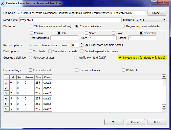
• Load the CSV file in QGIS


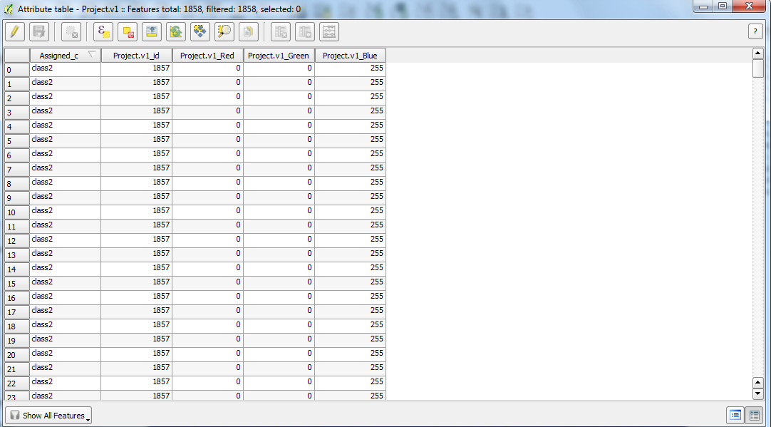
• Perform attribute Join of shape file and CSV file with key attribute join based on Class. With this you will get RGB values attached in attribute table of shape file.


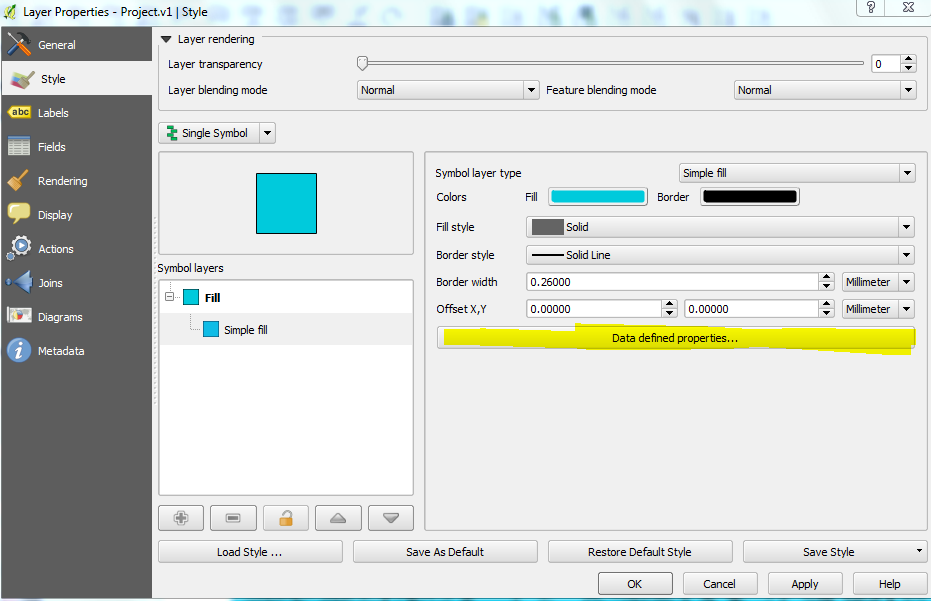
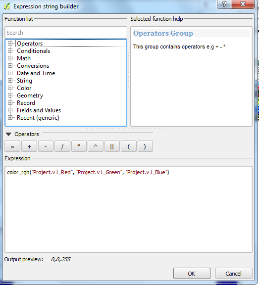
• Double click color symbology of shape file and use data defined properties of  color attributes  of shape file.


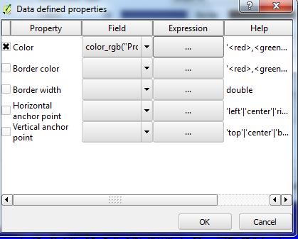
• Build an expression for color selecting respective color attribute column from shape file.

import CSV file into QGIS

Attribute of shape file after performing join

Data defined properties

data defined properties for color

data defined properties for color

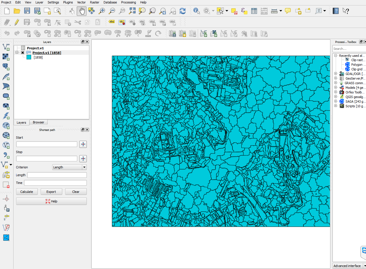
Normal display without color symbology

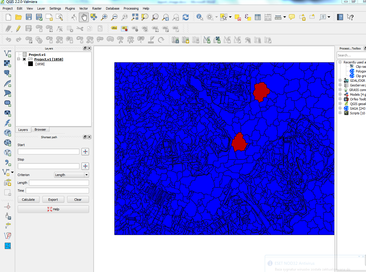
Display with color symbology

eCognition tutorial: Exporting eCognition features as images with array functionalities

There are instances when one would like to export different features from eCognition as a images to perform some tasks outside eCognition. eCognition doesn't provide a way to export many object features as images but it is only possible to export as a thematic raster in which each object has a unique ID, and features values are stored in a separated CSV file. To convert it into images, one has to mapped ID raster tiff file and data from CSV file.

If you want to get eCogntion features as images in an automatic way that can export any numbers of features as images in one go, then here is a way. For the purpose, we are going to utilize array handing capabilities of eCogntion and export each feature as separate tiff (My_1.tiff, My_2.tiff …. and so on) file. The rule set can be downloaded here. The rule set is flexible in the sense that you just have to update an array to store your feature list of interest. Number features can be any number (10, 20 or even 100 features). We will merge it afterwards in open source QGIS.

• Perform a segmentation
• Create a array and store features you want to export as images
• Loop over the array

1. For each feature, create a temporary image file
2. Export the temporary file as a unique name
3. Repeat until all features in the array are executed

• Now in QGIS, we use GDAL to stack individual images into one single image. We will use merge function of GDAL (Raster>Miscellaneous> Merge).

  

  Complete ruleset within eCognition

Ruleset  for exporting features as images 

GDALmerge function within QGIS

Color composite of three merge features

Thus produced merge features image now can be used for classification  in ENVI, ERDAS IMAGINE or writing custom script in Python or MATAB. Personally I use such images within Python using scikit-learn library.