Pages

Friday, 10 October 2014

QGIS tutorial: Display with color symbology from data defined properties of shape files


How many of you have this problem: you classify your images in ecognition or any other software and exported classified image as shape file. Now you want to view the shape file in a GIS environment and with the same color for each class that was used in eCognition. Manually matching color RGB values from eCognition to shape colors for each class is a tedious task, specially when  you have many classes.

This problem can be solved with a little trick.

  • Do your classification in eCognition. Assign class colors as you wish.

  • Export classification result as shape file with Class attributes.

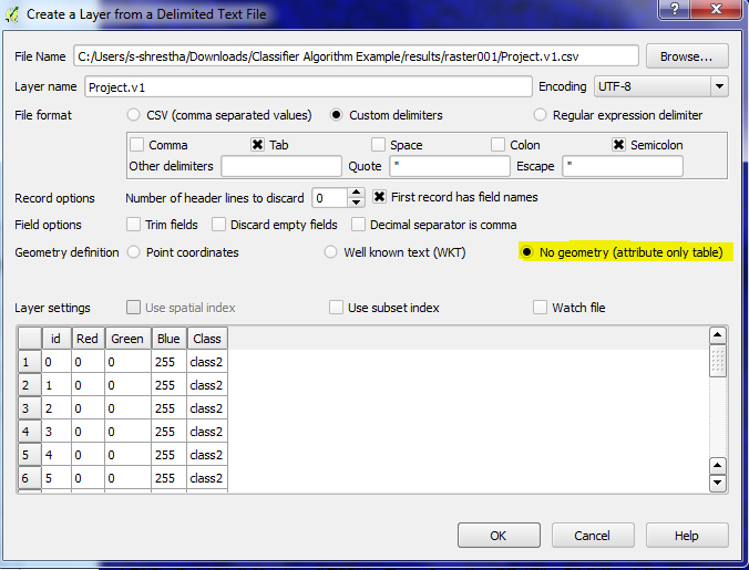
  • Export classification result as thematic raster. By doing so, you will get a CSV file in which you can get RGB color codes for each class.

  • Load your shape file in GIS (I use QGIS which is free. I am a poor guy therefore I always love free stuffs)

  • Load the CSV file in QGIS

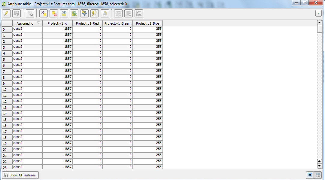
  • Perform attribute Join of shape file and CSV file with key attribute join based on Class. With this you will get RGB values attached in attribute table of shape file.

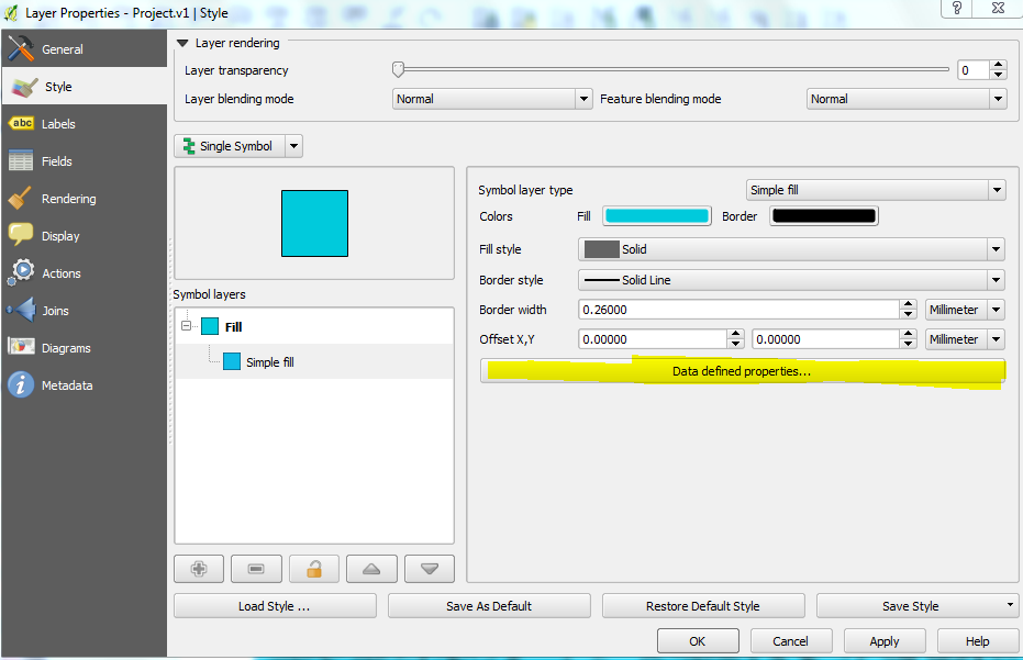
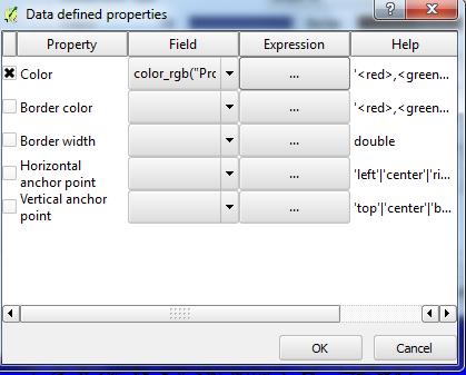
  • Double click color symbology of shape file and use data defined properties of  color attributes  of shape file.

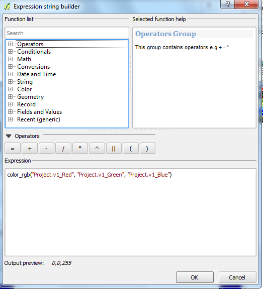
  • Build an expression for color selecting respective color attribute column from shape file.
import CSV file into QGIS

Attribute of shape file after performing join
Data defined properties
data defined properties for color

data defined properties for color
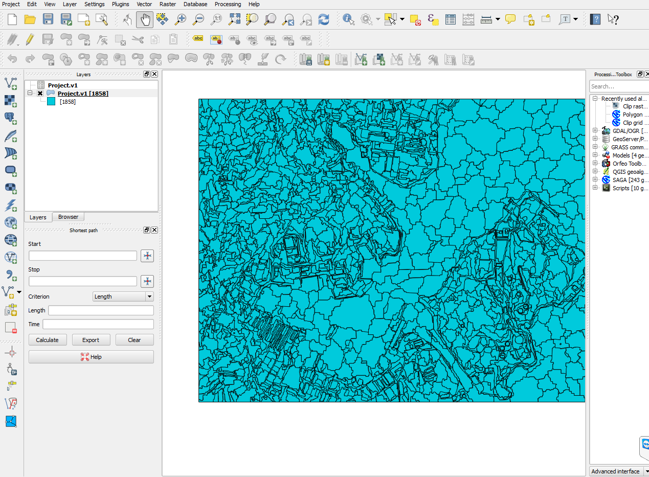
Normal display without color symbology

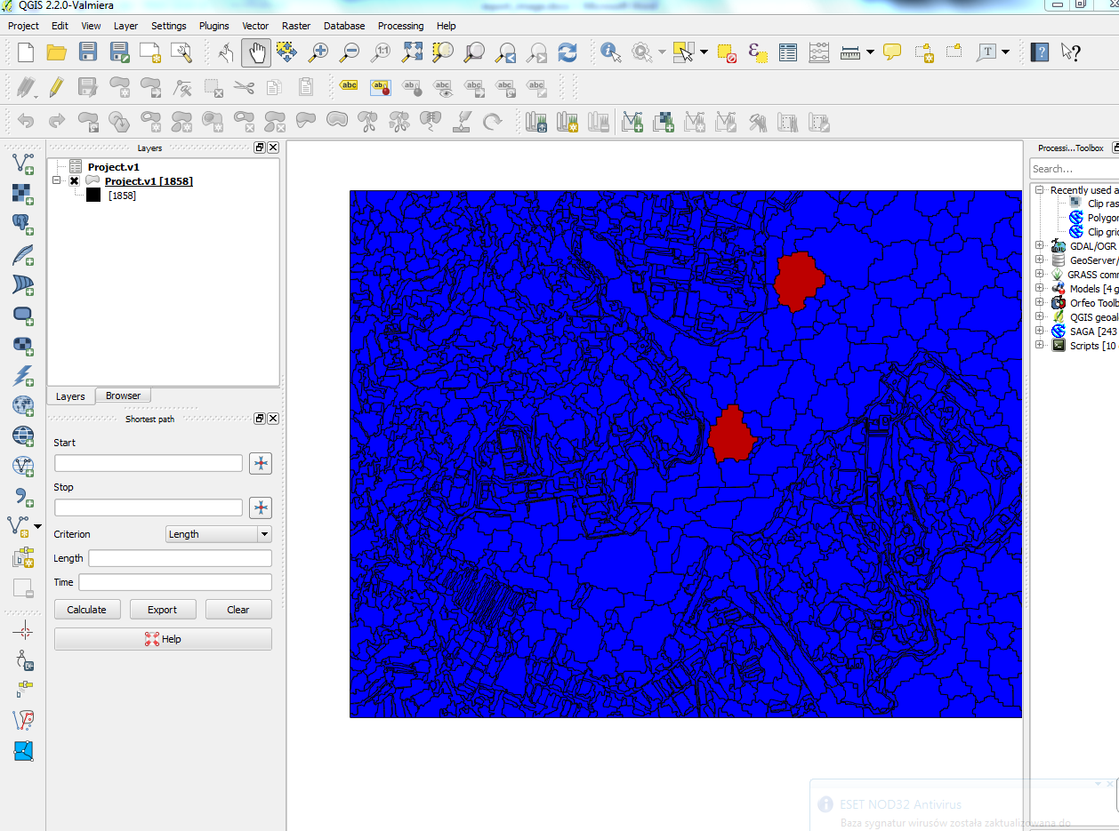
Display with color symbology


Wednesday, 8 October 2014

eCognition tutorial: Exporting eCognition features as images with array functionalities

There are instances when one would like to export different features from eCognition as a images to perform some tasks outside eCognition. eCognition doesn't provide a way to export many object features as images but it is only possible to export as a thematic raster in which each object has a unique ID, and features values are stored in a separated CSV file. To convert it into images, one has to mapped ID raster tiff file and data from CSV file.

If you want to get eCogntion features as images in an automatic way that can export any numbers of features as images in one go, then here is a way. For the purpose, we are going to utilize array handing capabilities of eCogntion and export each feature as separate tiff (My_1.tiff, My_2.tiff …. and so on) file. The rule set can be downloaded here. The rule set is flexible in the sense that you just have to update an array to store your feature list of interest. Number features can be any number (10, 20 or even 100 features). We will merge it afterwards in open source QGIS.

  • Perform a segmentation
  • Create a array and store features you want to export as images
  • Loop over the array
    1. For each feature, create a temporary image file
    2. Export the temporary file as a unique name
    3. Repeat until all features in the array are executed
  • Now in QGIS, we use GDAL to stack individual images into one single image. We will use merge function of GDAL (Raster>Miscellaneous> Merge).
    Complete ruleset within eCognition
Ruleset  for exporting features as images 
GDALmerge function within QGIS
Color composite of three merge features
Thus produced merge features image now can be used for classification  in ENVI, ERDAS IMAGINE or writing custom script in Python or MATAB. Personally I use such images within Python using scikit-learn library.

Friday, 15 August 2014

eCognition tutorial: Exporting eCognition classification file to ENVI

The problem:

I was wondering if anyone could help me export a usable file from eCognition Developer for use in ENVI 5.0? I've classified an image using Multiresolution Segmentation followed by the Classification algorithm using selected samples from the Standard Nearest Neighbour and everything worked so far. I try and export it as an ENVI-supported file type (e.g. *.tif) the raster seems to have "lost" all the classification- leaving a grayscale image- useless! I have been able to open a *.jpg file, but as it is an image it has lost any previous classfication from Ecognition.

Solution:

This is not even a problem but for people who are just starting with ENVI is a big HEADACHE. It’s just a matter of a symbology. If you have been using the ENVI for a while you should know that ENVI uses two files for any image. One binary file and another hdr file where different information about the binary image are stored. One can simply open hdr files with a notepad. Normal raster images have “file type = ENVI Standard” whereas classification images have “file type = ENVI Classification” and some other information such number of classes, class names and class colours. So the classified tiff file that one exports from eCognition does not have those information, hence ENVI opens the classified tiff file as a normal file. There are values differentiating classes but colour information are lost. This is a problem if you want to do some other operation in ENVI that required a classification image as input.

So we need to convert it ENVI Classification type, somehow. So here is a way to do it.

  1. Do your classification in eCognition.
  2. Export it using “export thematic raster files” algorithm in eCognition with Export Type Don’t forget to select your classes in Class Filter parameters
  3. Once you export it, you will have two files. One *.tiff file and other *.csv fil. Open *.csv file, there you will find class names and RGB colour for each class.
  4. Open *.tif file in ENVI.
  5. Then File> File Save as > ENVI Standard>Import file > Pick recently open tif file. Give a name and save it. Now you changed tiff file to ENVI file but remember, its still a normal ENVI standard file.
  6. Open the file created in step 5. Then File> Edit Header Info > Select File type as ENVI classification. It will prompt you for number of classes, class names, colour information. Provide those information by using *.CSV file that you opened in step 3.
  7.   Now you have a ENVI classification image with same class names and colour as in eCognition. Now smile and go for a coffee.

Example of a CSV file
Converting tiff file to ENVI file
Modifying header files
Editing class names and color information

Initial and Final image

Friday, 11 July 2014

Data exchange between MATLAB and Python: Reading and writing .mat fileswith Python

I am a MATLAB guy. I love MATLAB. I started with Fortan during my first degree at my Bachelor level. I came across with MATLAB only in year 2010 as a part of my Msc studies. Since then I been using it continuously for various tasks. Just recently, I started  using Python and I LOVE IT. The biggest reason being that Python is open-source and there are lots of Python libraries that can be used. But there are times; I have to shuffle data between MATLAB and python, because for some tasks I prefer MATLAB as I am accustom to it. So if you are in the same boat, then here I show you simple way to transfer data between MATLAB and Python. One has to use scipy.io module in Scipy for that purpose. If you have some old data or got some data online that are saved as MATLAB’s .mat file format, you can simply import it as:

import numpy as np
import scipy.io as sio
mydata = sio.loadmat('mydata.mat')

Now your mydata contains a dictinary with keys corresponding to the varible names saved in the original mydata.mat Saving a python variable to .mat file is also straight forward

# write one variable
x = np.arange(1,10,1)
# file name of the file
fname ='export_from_python.mat'
sio.savemat(fname, {'x':x})

When you read export_from_python.mat, you will get 'x' varialbe into MATLAB. If you want to write more than two variable:

# write two variables
x = np.arange(1,10,1)
y = np.ones((5,5))
fname ='export_from_python_1.mat'
sio.savemat(fname, {'x':x, 'y':y})

I do lot of work with classification of remote sensing images using many different types of machine learning algorithms. Proprietary software like ENVI and ERDAS are not flexible enough for me, as these software donot allow an efficient way to tune hyper-parameters that are algorithm specific. I dont like training models with defualt parameters. I do my model traning and classification in python. Here is the typical workflow.
  1.  Import image and training data in python using GDAL
  2. Train machine learning model in python using Sci-kit Learn
  3. For accuracy assessment, i do it within python but for accuracy assessment visualization, i export  targets and outputs vectors from Python to MATLAB
  4. Use 'plotconfusion' function from Neural Network toolbox for a visualization of confusion matrix. Here is the confusion Matrix  information that i got from MATLAB. Its nice, isnt it ?

Picture1
Confusion matrix

Friday, 7 February 2014

Example of extracting grid nodes in MATLAB

For last few posts, I am writing about morphological image analysis with python with open source package scikit-image. In this post I want to show benefit of morphological image analysis with some real application. I been working with road extraction from satellite images for past few weeks and  one of the common task is to extract the grid corner nodes of the road network. So let’s assume the road grid has been already extracted and we want to extract intersection of grid network. Here I am showing three approaches for that based on synthetic data. Obviously with real data, the task is more complex and might require many slight modifications.

Here is the grid. You can generate such grid with checkerboard function in MATLAB with minor processing (edge detection and hole filling). Intersections of of grid lines have a property that it has 4 white pixels in 4-N neighborhood.  We can exploit this property to extract it. I am going to show to ways by which it can be done and in addition, another method based on extraction of corners will also be shown.

%make a checkerboard
I=checkerboard(20, 10,10)>0.5;
imshow(I)
% detect edge with canny
BW = edge(I,'canny');
figure, imshow(BW)
%make square structural element to fill holes with closing
SE = strel('square', 3);
BW1 = imclose(BW, SE);
figure, imshow(BW1)
% make a skeleton of the to lines 1 pixel thick
BW2 = bwmorph(BW1,'skel',Inf);
figure, imshow(BW2)


1

 26


In mathematics and, in particular, functional analysis, convolution is a mathematical operation on two functions f and g, producing a third function that is typically viewed as a modified version of one of the original function .In simple word, convolution of image is a process where you scan your image from left to right and top to bottom within local neighborhood defined by user, and do mathematical calculation within the local neighborhood. Here we are going to use it for simply sum the number of pixels which are which are white within 3x3 neighborhood. As shown by above figure, if the point is an intersection grid point then at that point sum should be 5. Any points with less than 5 white pixels are not intersection grid points.

% with block processing and inline function with convolution
tic;
kernel = [0 1 0; ... %# Convolution kernel
1 1 1; ...
0 1 0];
sumX = conv2(double(BW2),kernel,'same');
result=sumX;
% only consider pixels which are in grid image
result (BW2==0)= 0
result(sumX<5)=0;
[r,c] = find(result>0);
toc;
figure,imshow((BW2)), hold on, plot(r,c,'r*');title ('with Convolution')
hold off
3
Way Two: With Mathematical Morphology (MM)
If you are working in the field of Geo-information and you still saying what the heck this ‘MM’ then seriously you should be acquainted with this field of image processing. You can use MM for classification, edge detection, filtering, segmentation, building detection and many other things. Grab a cup of coffee and Google MM in remote sensing; there is tons of stuff to read.  There are courses in MM taught in different universities which are one semester long, so you got an idea how vast the subject is. If you want to seriously know MM, then there is no better book than ‘ Morphological Image Analysis’ by P Soillie. Here we use ‘Erosion’ method of MM.  Time: 0.011184 seconds.

% method two with morphological analysis
tic;
SE = strel ('disk', 1);
result2 = imerode(BW, SE);
[r,c] = find(result>0);
toc;
figure,imshow((BW2)), hold on, plot(r,c,'b*'), title ('With MM Erosion')
hold off
4
Way Two:  Mathematical Morphology (MM)
There are many corner detection techniques such as Moravec, Harris, SIFT etc. Here, I am going to use Harris corner detector for intersection grid points. Time: 0.094848 seconds.

% detect corner by harris corner detector
tic;
C = corner(BW2,500 );
timet2 = toc;
toc;
figure,imshow(BW2);
hold on
plot(C(:,1), C(:,2), 'g*'); title('with harris corner detector')
hold off
5
Way Two:  With Harris Corner Detector
So you have seen there are number of ways to solve a particular problem. All above methods detected intersection points successfully. Among three methods, convolution required longest time for processing and MM required shortest time. The gain in computation cost between MM and Corner detection is 9 folds.  I did all this in MATLAB but it can easily coded in python with scikit-image.
Thursday, 23 January 2014

Example of Opening by reconstruction in scikit-image

This blog is a continuation of the last blog that I have written. The aim is to give you potential of the mathematical morphology (MM) using ski-image and their application.  MM is branch of image processing which has wide application in many diverse field. Erosion and dilation are basic operators of MM which can be combined in different way to form many different powerful MM operators. MM was devised for binary images but nowadays it has been extended to grayscale images as well.

Here I would show you application of erosion and opening by reconstruction to do some image processing. For definition of erosion and opening by reconstruction please follow any image processing books or look in the web there are many online tutorials.

So we have an image. Let us assume that out the different blobs that we have we want to have a blob which should have a minimum length of 200 pixels in horizontal direction. Such expert knowledge is handy in many images processing domain to improve the image analysis. E.g building cannot be less than certain width, road should be of certain width, bridge should be of certain width etc. in this case lets assume, the shown blobs are result of some building detection algorithm. Now we want to improve the result by incorporating expert knowledge using MM.

figure_4

So first we want to erode the image with linear structural element of length 200 pixels and whatever is remaining after that, we want to recover original shape of the blobs which was distorted by using erosion. For that purpose we use opening by reconstruction. Here are the codes, enjoy and dont forget to play around with python.

figure_5figure_6


# -*- coding: utf-8 -*-
Created on Mon Nov 18 15:42:21 2013
@author: shailesh
"""
#%%
% call necessary libraries
import math
import matplotlib.pyplot as plt
import numpy as np
from skimage.draw import ellipse
from skimage.draw import polygon
from skimage.draw import circle
from skimage.morphology import label
from skimage.measure import regionprops
from skimage.transform import rotate
import matplotlib.patches as mpatches
import skimage.morphology as MM
% draw some arbitary shapes
image = np.zeros((1000, 1000),dtype=uint8)
&nbsp;
% create an ellipse with centre (350,350) with minor axis = 100 and major = 220
rr, cc = ellipse(300, 750, 100, 220)
image[rr,cc] = 1
&nbsp;
&nbsp;
% create a polygon
x = np.array([1, 7, 4, 1])
x = np.array([1, 70, 40, 1])
y = np.array([1, 20, 80, 1])
rr, cc = polygon(y, x)
image[rr, cc] = 1
&nbsp;
% create a polygon
rr, cc = circle(200, 200, 50)
image[rr, cc] = 1
fig, ax = plt.subplots(ncols=1, nrows=1, figsize=(6, 6))
&nbsp;
&nbsp;
&nbsp;
rr, cc = ellipse(500, 800, 30, 40)
image[rr, cc] = 1
ax.imshow(image)
&nbsp;
#lable connected regions
label_img = label(image)
#find properties of connected regions
regions = regionprops(label_img,['Centroid','Area','BoundingBox'])
&nbsp;
%loop through connected regions and find
% Centroid', 'BoundingBox', 'Area' for each blobs
i= 0
&nbsp;
NOS= len(np.unique(label_img))-1
X = np.zeros((1,NOS))
Y = np.zeros((1,NOS))
&nbsp;
for props in regions:
y0, x0 = props['Centroid']
print x0, y0
%show figure
plt.gray()
plt.axis((0, 1000, 1000, 0))
plt.title('original image')
plt.show()
&nbsp;
%perform erosion with linear structuring element
SE= np.ones((1,200))
figure()
imageE = MM.binary_erosion(image, SE)
plt.imshow(imageE)
plt.title('Eroded image')
plt.show()
&nbsp;
figure()
%perform opening by reconstruction to recover blob
imageRECON = MM.reconstruction(imageE, image)
plt.imshow(imageRECON)
plt.title('Reconstructed image')
plt.show()

Morphological reconstruction is a very powerful method. People have use it for many different applications such as watershed delieanation, filtering, change detection of building after earthquakes, building detection, bridge detection etc. For my work also, i have used the technique for unsupervised change detection using high resolution images and change detection of high rise buildings.

Thursday, 5 December 2013

A little teaser for using scikit learn for classification of remotesensing images

I work with classification of remote sensing images a lot both with supervised as well as unsupervised classification. Unsupervised classifications don’t need any external input where as supervised classifications need samples or training areas for an algorithm to learn. For processing remote sensing images, there are many proprietary software like ENVI, ERDAS, PCI Geomatica, Global Mapper, eCognition and many more. Even after paying thousands of Euros, classifications algorithm available in Costs-off-the-self (COTS) software is far from satisfactory.

  • Software
  • Available Algorithms
  • eCognition 8.7

  • (cost >1000 Euros/year)

  • KNN

  • Decision Tree DT

  • SVM (no Y and C parameters available for tunning, no way to perform grid search for optimal determination of Y and C, Only linear and rbf kernel available)

  • Random Forest  RF (only available in 8.8
  • ENVI

  • (cost >1000 Euros/year)

  • Maximum Likelihood (ML)

  • SVM (no way to perform grid search for optima, unless you get your hands dirty with IDL programming

  • Neural Network NN ( Numbers of hidden nodes cannot be assigned)

  • Some otheralgorithms more suitable for Hyperspectral imagesy

  • SAM, SID, Spectral Unmixing.
  • Scikit learn

  • Free

  • Opensoure

  • Neighrest Neigbour (NN)

  • Decision Tree (DT)

  • SVM ( Grid search, cross validation flexibility)

  • Random Forest RF

  • AdaBoost

  • Naives Bayes

  • Linear Discriminant Analysis (LDA)

  • Quadratic Discriminant Analysis (QDA)


Here is the little teaser of classification accuracy with many algorithms that are available in scikit-learn for a remote sensing imagery. In near future, I will blog with more illustration and with code. Till then go and make your hands dirty with Python and Scikit-Learn. Make that your new year resolution and trust me, you will thank me for that.

Accuracy1

Here, algorithms hyperparameters were not optimally tuned hence superior machine learning algorithms like SVM has very low accuracy for test samples which are not seen by trained model.