eConition Tutorial: Customized algorithm for performing majority vote in eCognition

Today, I present you a customized rule set which lets you to assign super-object by evaluating all of its sub-objects based on which classification makes up the largest proportion of the area. This is one of the wishlist in eCognition Ideas and was also frequently asked in the ecognition community.

A majority statistic customized algorithm lets you assign  super- object to the class with the majority value of the pixels within each object. This would be useful for converting existing pixel-based classifications into an object-based format where additional object-based edits can be made.

The only parameter in this customized algorithm is a level variable. This is a level which consists of super-object. The customized algorithm will look one level below the level variable and perform all the necessary calculation.

Sub-objects level with classification

Super-objects level with no classification

Super-object level with classification from customized algorithm

The customized algorithm does assignment of super-object with following steps.

1) store all the classes in an array ( array_class)
3) loop through your objects in super objects
2) loop through your class arrays
4) store rel. area of (1) in an array for the class ( array_occur)
5) find maximum in the array_occur
6) assign super-object as maximum occurrence class in array  array_occur.

All of these steps are performed behind the scene in customized algorithm, so the user does not need to worry about how to perform these steps.

I have uploaded a zip file where you will find a project which shows the usage of the customized algorithm. There is a  customized rule-set as well. Load the customized rule set in your project and after that you will find a algorithm MajorityVote in the available algorithm list.

The algorithm was developed with eCogntion 8.8 and  will not work below that version.

eCognition tutorial: Customized algorithm for performing majority vote in eCognition

Today, I present you a customized rule set which lets you to assign super-object by evaluating all of its sub-objects based on which classification makes up the largest proportion of the area. This is one of the wishlist in eCognition Ideas and was also frequently asked in the ecognition community.

A majority statistic customized algorithm lets you assign  super- object to the class with the majority value of the pixels within each object. This would be useful for converting existing pixel-based classifications into an object-based format where additional object-based edits can be made.

The only parameter in this customized algorithm is a level variable. This is a level which consists of super-object. The customized algorithm will look one level below the level variable and perform all the necessary calculation.

Sub-objects level with classification

Super-objects level with no classification

Super-object level with classification from customized algorithm

The customized algorithm does assignment of super-object with following steps.

1) store all the classes in an array ( array_class)
3) loop through your objects in super objects
2) loop through your class arrays
4) store rel. area of (1) in an array for the class ( array_occur)
5) find maximum in the array_occur
6) assign super-object as maximum occurrence class in array  array_occur.

All of these steps are performed behind the scene in customized algorithm, so the user does not need to worry about how to perform this steps.

I have uploaded a zip file where you will find a project which shows the usage of the customized algorithm. There is a  customized rule-set as well. Load the customized rule set in your project and after that you will find a algorithm MajorityVote in the available algorithm list.

The algorithm was developed with eCogntion 8.8 and  will not work below that version.

Setting up object based change detection rule set in Ecognition

I have been very busy lately, so apologies. But on the flip side I am writing something that may be useful for many of you. eCognition is pioneer software for doing object based image classification.  Let’s say, you have two images classified, time T1 and time T2 and you want to identify change and no change areas.

Time T1

Time T2

Change/ No Change map to be produced

You would proceed like this:

1)      Copy Map T1 to Map Change detection in lvl T1

2)      Copy lvl T1 above and name as lvl T2

3)      Synchronize Maps T2 with lvl T2 in Map Change Detection.

4)      At lvl T2Ł convert to sub object

5)       Copy lvl T2 in Map Change Detection.above and name as lvl change

6)      Delete classification in lvl change

By doing these steps, you have a level, lvl change where each object is of same size as in the sub objects  in lvl T1 and lvl T2. Now you want to classify objects in lvl change as change and no change. How would you proceed?

Majority of people proceed like this:

1)      Set up a class No change, and look for change in class for each objects  using ‘Existence of sub object”’ in sub objects in lvl T1 and lvl T2 (c.f. figure).  Figure shows set up of rule set for one class only.

Class description when one class only 

2)       Generally classification has many numbers of classes. When adding one more class in the rule, the class description of No change class becomes a bit complex.

Class description when two classes only 

3)      Now imagine you have 20 different classes. Of course you can perform the process by adapting the rule description for No change for another 18 class. But it’s a tedious process and takes time. Further, the same class description cannot be used for another set of classification maps which may have different class names.So what would you do in this case?

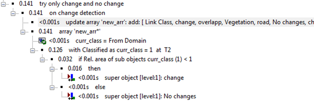
4)      Wise, things to do is to take benefit of array handlings capabilities of eCognition, concept of sub-object, super-object and Parent Process Object (PPO).I am showing you a solution that is short and does not need any set up of class description in change and No change class, easily adaptable to other projects.

6)      I leave up to you to try to understand the rule set shown above. If you don’t understand, give me a shout, I will try to explain.

eCognition tutorial: Setting up object based change detection rule set in Ecognition

I have been very busy lately, so apologies. But on the flip side I am writing something that may be useful for many of you. eCognition is pioneer software for doing object based image classification.  Let’s say, you have two images classified, time T1 and time T2 and you want to identify change and no change areas.

Time T1

Time T2

Change/ No Change map to be produced

You would proceed like this:

1)      Copy Map T1 to Map Change detection in lvl T1

2)      Copy lvl T1 above and name as lvl T2

3)      Synchronize Maps T2 with lvl T2 in Map Change Detection.

4)      At lvl T2Ł convert to sub object

5)       Copy lvl T2 in Map Change Detection.above and name as lvl change

6)      Delete classification in lvl change

By doing these steps, you have a level, lvl change where each object is of same size as in the sub objects  in lvl T1 and lvl T2. Now you want to classify objects in lvl change as change and no change. How would you proceed?

Majority of people proceed like this:

1)      Set up a class No change, and look for change in class for each objects  using ‘Existence of sub object”’ in sub objects in lvl T1 and lvl T2 (c.f. figure).  Figure shows set up of rule set for one class only.

Class description when one class only 

2)       Generally classification has many numbers of classes. When adding one more class in the rule, the class description of No change class becomes a bit complex.

Class description when two classes only 

3)      Now imagine you have 20 different classes. Of course you can perform the process by adapting the rule description for No change for another 18 class. But it’s a tedious process and takes time. Further, the same class description cannot be used for another set of classification maps which may have different class names.So what would you do in this case?

4)      Wise, things to do is to take benefit of array handlings capabilities of eCognition, concept of sub-object, super-object and Parent Process Object (PPO).I am showing you a solution that is short and does not need any set up of class description in change and No change class, easily adaptable to other projects.

6)      I leave up to you to try to understand the rule set shown above. If you don’t understand, give me a shout, I will try to explain.

Opening multispectral or hyperspectral ENVI files in MATLAB

ENVI/IDL is one of the most used remote sensing software package which has a nice programming interface known as IDL. Though I have been using IDL for quite some time now, I still prefer MATLAB over IDL because MATLAB has extensive help documentation with lots of useful demonstration which I think is lacking in IDL.

There is a function in MATLAB which not many people are aware of, which is called Multibandread. Multibandread can be use for any type of binary files such as bsq, bil and bip. As long as you know how the data is organized in the binary file, its data type, rows columns and no. of bands in the file you can read the file in MATLAB with Multibandread.  Multibandread requires following informations.

X = multibandread(filename, size, precision, offset, interleave, byteorder)

With ENVI files, you can find all these information in the header file of that ENVI file. Using that information, you can pass this information by manually typing or you can write a custom function which will open the header file, fetch those information from the header file and pass it to Multibandread. I usally do it with latter approach.

Opening whole remote sensing images in MATLAB is a bit tricky. Consider you have a hyperspectral data with 116 bands and you try to read whole image at one go. MATLAB will run out of memory. The wise thing is to read the image in a block by block (MxN), performing required operation in the block and later combining all blocks. 

One cautionary note, I have seen people doing some silly mistakes such as reading an ENVI file with 10 bands in a variable (image) and using imshow (image) to visualize it. They spend countless hours wondering why the Multibandread is not being able read their ENVI files. But they forget that imshow function can display only three band one time. So if you want to view first three band then you have to use

  Imshow( image(:,:,1:3),[])

So, try Multibandread function if you are MATLAB savvy person and prefer MATLAB over IDL.

If you run into any kind of problem, I am ready for help.

Utilizing Numpy to perform complex GIS operation in ARCGIS 10

Today my country Nepal played with Jordan for securing  a place in world cup 2014 qualification. I was hoping for at least a draw but after 20 minutes or so, Nepal was already 3-0 down. I could not follow the live update anymore, therefore decided to grab a beer and  write something for my blog.This is how this post came into existence.

I wanted to write about array manipulation within a arcgis for a long time. The idea came from a problem that was faced by one of my close senior friend who  frequently uses  arcgis in his work. He had a raster (SRTM ) data and he wanted to calculated maximum value in a varying window ( like 5X5, 7X7, 9X9) for the data and marked that maximum value in the window as one. Focal statistics function in arcgis can calculated maximum value in a specified neighborhood but it assigns the maximum value in the centre cell. It does not tell where the maximum value lies within the window. So he asked me for suggestion, and I , being a MATLAB savvy person quickly wrote a function in MATLAB which would do the trick. I send the solution to the friend but the problem was, he was not familiar to MATLAB and he did not have access to MATLAB as well. He wanted to have a solution that works within the arcgis.

So, I have dived into NUMPY which is a fundamental package in Python for large, multi-dimensional array and matrices for solving the problem. It is already integrated into arcgis 10. In arcgis 10, there are two functions namely RasterToNumPyArray and NumPyArrayTORaster. First function converts a raster to matrix and second function converts a matrix to array. These two functions open a new opportunity for performing MATLAB like matrix manipulation within the arcgis.

So, in this post I will show you how problem mentioned before can be solved. First I will show you the code and will explain it concisely.

1. import arcpy


2.  from numpy import *


3. myArray = arcpy.RasterToNumPyArray('basic_raster')


4. [cols,rows]= myArray.shape


5.  winsize= 3;


6.  winhalf = 1


7.  I=zeros((cols, rows))


8.  for n in range(winhalf,rows-winhalf):


9. for m in range (winhalf,cols-winhalf):


10. data = myArray[m-winhalf:m+winhalf+1,n-winhalf+1:n+winhalf+1]


11. maxdata = data.max()


12. indices = where(data ==maxdata)


13.  I[m-winhalf+indices[0],n-winhalf+indices[1]] = 1

Line 1 and Line 2 imports the arcpy and numpy module.

Line 3 stores raster ‘basic_raster’ in a variable myArray

Line 4 stores size of the matrix myArray

Line 5 defines a window size ( three in this case)

Line 6 creates a matrix which is same size of rater ‘basic_raster’ but all filled with zero

Line 8-13 does the main computation. It will iterate through 3X3 window and calculates the maximum value and assigns 1 to the location of cell which contains the maximum value in the window.

Now we could already exports the I matrix using the function NumPyArrayTORaster (I). But doing so has couple of disadvantage because by doing so we would have just exported the matrix as a raster without any information about the cell size, coordinate and projection information. Therefore we need to get all these information from ‘basic_raster’ which is the raster based on which we calculated matrix I. For this we can use a bit of arcpy.

14 descData=arcpy.Describe('basic_raster')
15 cellSize=descData.meanCellHeight
16 extent=descData.Extent
17 spatialReference=descData.spatialReference
18 pnt=arcpy.Point(extent.XMin,extent.YMin)
19 newRaster = arcpy.NumPyArrayToRaster(I,pnt, cellSize,cellSize)

Line 14 uses a function ‘Describe’ to get information about the raster ‘basic_raster’.

Line 15-18 stores different information in various variables

Line 159transforms matrix I into a raster named ‘newraster’ using information from the raster ‘basic_raster’

Now we have a new raster where one represents cells with a maximum values in a sliding window of 3x3 which perfectly aligns with the raster ‘basic_raster’ in the same projection system.

I hope you have gained some insights into enormous advantage of integrating numpy and arcpy in your GIS workflow. If you have some prior programming knowledge, you would find pretty easy to learn python. Even if you don’t have any programming experience, I suggest you to gets your hands dirty with python. It’s not that hard to learn python, believe me :).

Utilizing Numpy to perform complex GIS operation in ARCGIS 10

Today my country Nepal played with Jordan for securing  a place in world cup 2014 qualification. I was hoping for at least a draw but after 20 minutes or so, Nepal was already 3-0 down. I could not follow the live update anymore, therefore decided to grab a beer and  write something for my blog.This is how this post came into existence.

I wanted to write about array manipulation within a arcgis for a long time. The idea came from a problem that was faced by one of my close senior friend who  frequently uses  arcgis in his work. He had a raster (SRTM ) data and he wanted to calculated maximum value in a varying window ( like 5X5, 7X7, 9X9) for the data and marked that maximum value in the window as one. Focal statistics function in arcgis can calculated maximum value in a specified neighborhood but it assigns the maximum value in the centre cell. It does not tell where the maximum value lies within the window. So he asked me for suggestion, and I , being a MATLAB savvy person quickly wrote a function in MATLAB which would do the trick. I send the solution to the friend but the problem was, he was not familiar to MATLAB and he did not have access to MATLAB as well. He wanted to have a solution that works within the arcgis.

So, I have dived into NUMPY which is a fundamental package in Python for large, multi-dimensional array and matrices for solving the problem. It is already integrated into arcgis 10. In arcgis 10, there are two functions namely RasterToNumPyArray and NumPyArrayTORaster. First function converts a raster to matrix and second function converts a matrix to array. These two functions open a new opportunity for performing MATLAB like matrix manipulation within the arcgis.

So, in this post I will show you how problem mentioned before can be solved. First I will show you the code and will explain it concisely.

1. import arcpy
2.  from numpy import *
3. myArray = arcpy.RasterToNumPyArray('basic_raster')
4. [cols,rows]= myArray.shape
5.  winsize= 3;
6.  winhalf = 1
7.  I=zeros((cols, rows))
8.  for n in range(winhalf,rows-winhalf):
9. for m in range (winhalf,cols-winhalf):
10. data = myArray[m-winhalf:m+winhalf+1,n-winhalf+1:n+winhalf+1]
11. maxdata = data.max()
12. indices = where(data ==maxdata)
13.  I[m-winhalf+indices[0],n-winhalf+indices[1]] = 1

Line 1 and Line 2 imports the arcpy and numpy module.

Line 3 stores raster ‘basic_raster’ in a variable myArray

Line 4 stores size of the matrix myArray

Line 5 defines a window size ( three in this case)

Line 6 creates a matrix which is same size of rater ‘basic_raster’ but all filled with zero

Line 8-13 does the main computation. It will iterate through 3X3 window and calculates the maximum value and assigns 1 to the location of cell which contains the maximum value in the window.

Now we could already exports the I matrix using the function NumPyArrayTORaster (I). But doing so has couple of disadvantage because by doing so we would have just exported the matrix as a raster without any information about the cell size, coordinate and projection information. Therefore we need to get all these information from ‘basic_raster’ which is the raster based on which we calculated matrix I. For this we can use a bit of arcpy.

14 descData=arcpy.Describe('basic_raster')
15 cellSize=descData.meanCellHeight
16 extent=descData.Extent
17 spatialReference=descData.spatialReference
18 pnt=arcpy.Point(extent.XMin,extent.YMin)
19 newRaster = arcpy.NumPyArrayToRaster(I,pnt, cellSize,cellSize)

Line 14 uses a function ‘Describe’ to get information about the raster ‘basic_raster’.

Line 15-18 stores different information in various variables

Line 159transforms matrix I into a raster named ‘newraster’ using information from the raster ‘basic_raster’

Now we have a new raster where one represents cells with a maximum values in a sliding window of 3x3 which perfectly aligns with the raster ‘basic_raster’ in the same projection system.

I hope you have gained some insights into enormous advantage of integrating numpy and arcpy in your GIS workflow. If you have some prior programming knowledge, you would find pretty easy to learn python. Even if you don’t have any programming experience, I suggest you to gets your hands dirty with python. It’s not that hard to learn python, believe me :).